Next: Nucleotide substitution models implemented
Up: Nucleotide substitution models
Previous: A Markov model of
Contents
Transition matrices
The mathematical expression of a DNA Markov model uses a matrix  of substitution rates in which each element
  represents
the rate of substitution from nucleotide
represents
the rate of substitution from nucleotide  to nucleotide
  .
The diagonal elements of the
instantaneous rate matrix must satisfy the equation
.
The diagonal elements of the
instantaneous rate matrix must satisfy the equation
 |
(1) |
so that each row of sums to zero.
The process must be homogeneous and stationary; if  ,
,  ,
,  and
and
 are the four equilibrium bases frequencies then the rates must obey
the following constraint:
are the four equilibrium bases frequencies then the rates must obey
the following constraint:
 |
(2) |
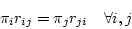
also known as the time-reversibility constraint. To enforce this constraint we define
 so that
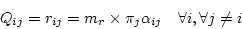 |
(3) |
where  is a constant factor described later. The time-reversibility
condition is satisfied with a symmetric choice of
is a constant factor described later. The time-reversibility
condition is satisfied with a symmetric choice of  . In practice,
PHASE
uses one of these parameters as a reference and sets its
value to
. In practice,
PHASE
uses one of these parameters as a reference and sets its
value to  . Depending on the model, other parameters (we call them
rate ratios) are fixed or inferred during an analysis.
. Depending on the model, other parameters (we call them
rate ratios) are fixed or inferred during an analysis.
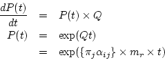
With we can compute the transition probability matrix over
time![[*]](./icons/footnote.png)
 .
.
The transition probability matrix
 is used to compute the
probability that nucleotide will be nucleotide after time
( can be equal to ).
The ``rate ratios'' matrix in PHASE
refers to
the matrix
and the ``transition rates'' matrix refers
to .
is used to compute the
probability that nucleotide will be nucleotide after time
( can be equal to ).
The ``rate ratios'' matrix in PHASE
refers to
the matrix
and the ``transition rates'' matrix refers
to .
Inference methods used do not permit the separation
of  , a factor proportional to the average substitution rate of the model,
and , branch lengths of the evolutionary tree which reflect an amount of change. The longer
the branch, the bigger the evolutionary distance between its two incident nodes.
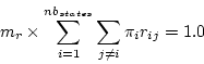
We have to impose a scaling on the branch length. In practice, we fix the
average rate of substitutions of our model to be one per ``unit of time''. This
is done by adding a constraint for the factor .
, a factor proportional to the average substitution rate of the model,
and , branch lengths of the evolutionary tree which reflect an amount of change. The longer
the branch, the bigger the evolutionary distance between its two incident nodes.
We have to impose a scaling on the branch length. In practice, we fix the
average rate of substitutions of our model to be one per ``unit of time''. This
is done by adding a constraint for the factor .
 |
(4) |
This last constraint does not hold when multiple substitution models are used
simultaneously in the MIXED model. The average substitution rate of
the first model is still fixed equal to 1.0 but the average substitution rate
of other models is now a free parameter.
Next: Nucleotide substitution models implemented
Up: Nucleotide substitution models
Previous: A Markov model of
Contents
Gowri-Shankar Vivek
2003-04-24